Introduction #

This course provides a brief introduction to parallel computing. It focuses on those paradigms that are prevalent in scientific computing in academia. There are other parallel programming models which we will mention in passing where appropriate.

Task

I think I have arranged for you to have a Hamilton account. Follow the instructions in that guide to log in and check that you can access Hamilton.

If you can’t access Hamilton, get in touch with me!

If you have a COSMA account, you can use that instead, and therefore need not use Hamilton.

Programming languages #

This course requires that you know, and can program in, C. If you’re used to high-level languages like Python, this can be a bit of a struggle when first starting. For a very brief “orientation” to the ways in which C differs from other languages, I recommend Simon Tatham’s descent to C. For a textbook, I recommend K&R, of which there are a number of copies in the library.

Why parallel computing? #

Computing in parallel is more difficult than computing in serial. We often have to write more code, or use more complicated libraries. If we are going to commit to doing it, there must be some advantage.

Our goal when running scientific simulations or data analyses is often to increase the resolution of the simulation, run more replicates (for example more bootstrapping samples in a statistical test), obtain answers faster, or some combination thereof.

In some cases, we might be analysing or simulating such high-resolution data that it does not fit in the memory of a single computer. Or, the problem may take so long that running it one a single computer would require us to wait a week or longer for the result.

For example, the UK Met Office produces a number of weather forecasts for the UK at various resolutions multiple times a day. This includes an hourly run making predictions for the next 12 hours. At the very least, a forecast is useless if it is slower than real time, and the target here is that every 12 hour forecast runs in under one hour (more than 12x real time). The model over the UK is at a resolution of 1.5km. This produces a computer problem that is large enough that each run is parallelised across 500 compute cores (so that they can hit their operational window of taking less than one hour to produce a forecast). To do this, the data, and algorithmic work that produce the model answers must be split up across these processes.

A perhaps simpler example comes when performing various forms of Monte Carlo integration. Of which we will see a very simple example in one of the exercises. The accuracy of Monte Carlo estimators increases when we add more samples. These samples are often completely independent. If we want to generate more samples (to improve accuracy), we can do so by running a single process code for longer, or dividing up the work of generating samples among multiple processes.

Moore’s Law #

The number of transistors in an integrated circuit doubles about every two years.

This was an observation Gordon Moore made about the complexity of chips in the mid-60s. That is, every 18-24 months, the computational performance available at a fixed price doubles.

This trend can be observed when we look at the performance of systems in the Top 500, which has been measuring the floating point performance of the largest 500 supercomputers in the world since 1993.

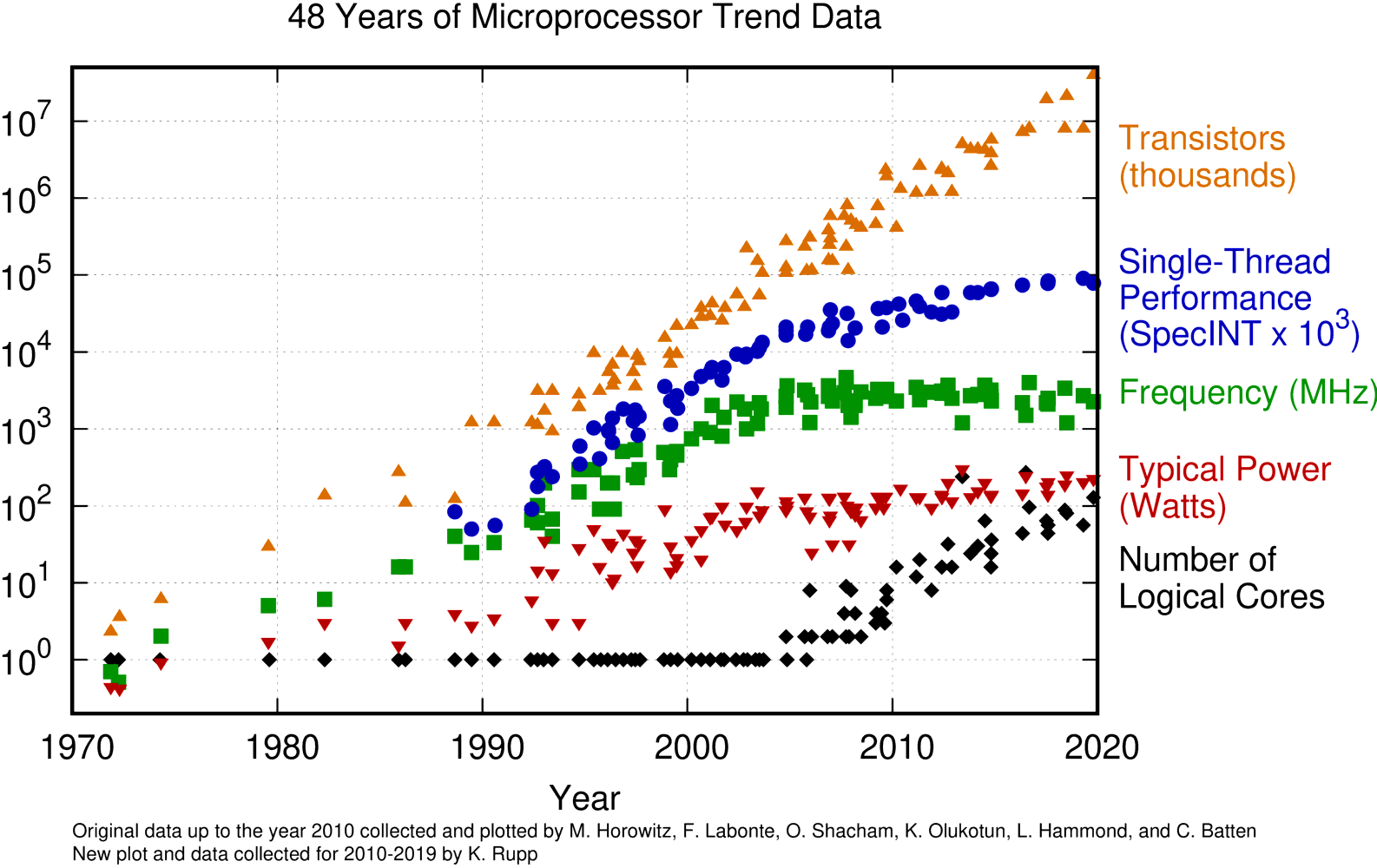
This seems great, however, there is a catch. If we zoom in and look at a history of CPU trends we see a slightly different picture.

Although the transistor counts still follow an exponential growth curve, CPU clock speed stopped increasing in around 2004. As a consequence, the single thread (SpecINT in the above figure) performance of modern chips has almost flat-lined since 2008. This Herb Sutter makes some nice observations about this in The Free Lunch is Over.

Exercise

Read The Free Lunch is Over. Make a note of what you think the key points are, and anything you didn’t understand, to bring to the live sessions.

Consequences #

If the number of transistors continues to increase, but the effective single-thread performance of CPUs does not (or at least, does not at the same rate), what are all these extra transistors being used for?

The answer is that they are used to provide parallelism. Notice how since 2004, the number of logical cores on a CPU has risen from one to typically around 32.

The consequence for us as programmers is that to use all the performance that chips provide, we must write code that exposes and uses parallelism.

Where next? #

We’ll introduce the different types of parallelism offered by modern supercomputers, and look at potential programming models and parallelisation strategies.